Damian Rezaee

Destination Toronto’s “You Gotta See What We See” campaign used TikTok videos, creator partnerships, and interactive ads that let viewers choose what to explore, such as dining, arts, or activities. TikTok’s case study reports 3.4 million unique reach, a click-through rate 296% above benchmark, and digital billboard impressions 44% above projections. Its page says the effectiveness claims are brand-reported and not verified by TikTok (TikTok for Business, n.d.).

Those are campaign-level results. Imagine the team then examining performance by creator, video, story choice, audience age, placement, and other factors. One subgroup appears to have an especially high click-through rate. That could point to a useful insight. It could also be the most striking result among many comparisons. The public case study does not say that Destination Toronto searched for a winning subgroup or that its reported results are unreliable. The example shows how easily a modern campaign can create many opportunities to find an eye-catching pattern.

In statistics, this problem is known as the look-elsewhere effect. It deserves more attention in marketing analytics, where teams can search through a great deal of data before deciding which finding to present.

What the look-elsewhere effect means

The term comes from particle physics. When researchers search for a new particle, they may not know in advance where it will appear in the data. They scan across a range of possible masses, looking for a signal. A bump at one precise mass may look unlikely under the assumption that no particle is there. The interpretation changes when researchers consider that they searched many possible masses and could have found a bump somewhere by chance. The relevant question is how unlikely a bump of this size would be anywhere in the range searched (Gross & Vitells, 2010; Lyons, 2008).

That distinction separates a local result from a global one. A local probability asks how surprising the result would be at the particular point where it appeared. A global probability also accounts for the search that led researchers to that point. The difference is sometimes described as a trial factor: the more opportunities there were to find an apparent signal, the less surprising the winning result may be.

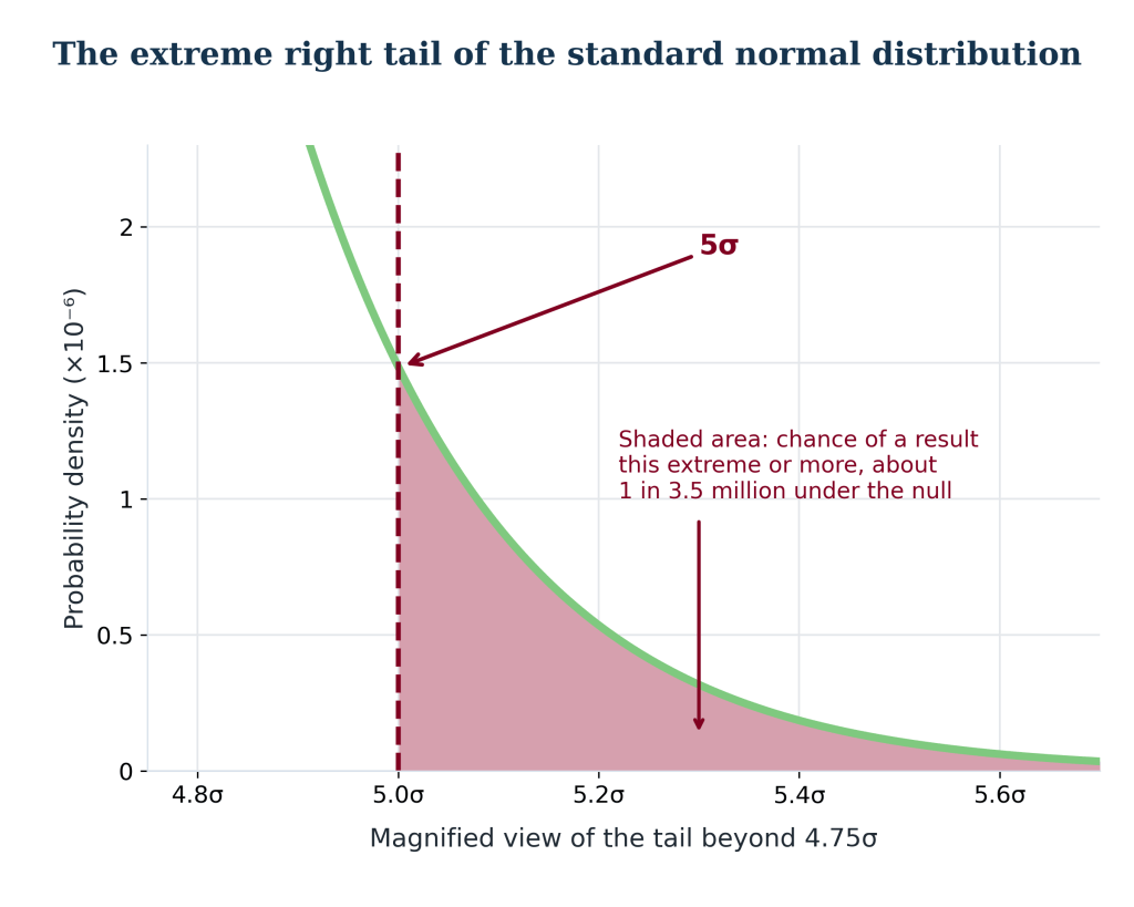
Particle physicists use a very strict five-sigma convention for claiming a discovery. A five-sigma result corresponds to roughly a one-in-3.5-million chance of a fluctuation under the null hypothesis. That convention is related to the look-elsewhere effect, but the two are distinct. Researchers also report global significance, which accounts for the range searched. In 2012, ATLAS reported a local significance of 5.9 sigma and a global significance of 5.1 sigma for its Higgs-like signal (ATLAS Collaboration, 2012).

Marketing teams face the same problem in a different setting. They search across audiences, channels, time periods, campaign versions, and outcomes. If they report only the strongest result, its apparent strength can be misleading unless they also account for how it was found.

Why one striking result is easy to find

Suppose an analyst runs one statistical test at a 5% significance level. If there is no real effect and the test’s assumptions hold, the chance of a false positive is 5%. If the analyst runs 20 independent tests under the same conditions, the probability of at least one false positive is about 64%. With 100 independent tests, it is about 99.4%.

The calculation is , where m is the number of independent tests. Real marketing comparisons are often related to one another, so the formula does not describe every analysis exactly. Comparing neighbouring age groups, for instance, is not the same as running completely separate tests on unrelated samples. Still, the underlying point holds: more searching creates more chances to find a result that looks convincing by accident.

This does not mean that a reported result is automatically false. It means the evidence is weaker than it appears if the analysis presents the winning comparison as though it were the only one considered. A p-value answers a specific question about a test under stated assumptions. It does not tell the reader how many other possibilities were explored before that test was selected.

Why marketing analysis is especially exposed

Marketing data makes exploration easy. An analyst can filter a dashboard by audience, device, channel, geography, creative, purchase history, or date range in seconds. Each new view can feel like a sensible follow-up question. The difficulty is that those choices accumulate. A final report may show one segment and one metric, while the analysis that produced it involved many discarded cuts and comparisons.

This resembles what Gelman and Loken (2014) call the “garden of forking paths.” Researchers can make a series of reasonable choices in response to the data, with each choice shaping what they look at next. The final path can then appear more planned and singular than it really was. Simmons et al. (2011) similarly showed how flexibility in measurement, data collection, and analysis can increase the chance of false-positive findings. In marketing, the flexibility may arise through decisions about which customer groups to compare, which dates to include, how to handle outliers, which metric to emphasize, and when to stop examining the results.

Dashboards can make this search hard to notice. A formal statistical test is easy to count; a series of filters may not feel like testing at all. Yet if the team examines many combinations and chooses the one that supports a decision, the search process matters even if no one set out to “fish” for a result.

Time adds another dimension. Teams often check campaign results every day and stop when the numbers look promising. If they use a standard fixed-sample test while repeatedly checking the data, the chance of a false positive can increase. Sequential methods are designed for ongoing monitoring, but the stopping rule has to be part of the method rather than an informal response to whichever day looks best (Johari et al., 2017).

The same issue appears when teams measure several outcomes. A campaign might be judged on clicks, conversions, revenue per user, repeat purchases, retention, and brand lift. If the primary outcome is disappointing, a secondary measure may become the headline. A result can still be informative, but it should be described as exploratory if the team chose to emphasize it after seeing the data. Kerr (1998) uses the term “HARKing” for building a hypothesis after the results are known and presenting it as if it had been predicted in advance.

There is also a reporting problem. Successful or surprising results are easier to turn into a presentation than null results. When unremarkable analyses disappear from view, colleagues and decision makers see a record filled with apparent wins. Rosenthal (1979) called a related research problem the “file drawer problem”: studies that find no effect are less likely to be published. Inside an organization, the equivalent may be the campaign analysis that never becomes a case study because it produced no story. Without a record of what was tested and what was found, teams cannot judge how often their reported discoveries are likely to be false leads.

Weak effects make the search more treacherous

Advertising effects can be difficult to measure because the change generated by a campaign may be small compared with the ordinary variation in sales. Lewis and Rao (2015) examined 25 large field experiments with major U.S. retailers and brokerages, most of which reached millions of customers. They found that the median confidence interval for return on investment across the experiments was over 100 percentage points wide.

This measurement challenge matters when teams search across many possible effects. If most campaign changes have little or no impact, then a long list of tests will contain many null effects. Some comparisons will still look unusually strong by chance. Ioannidis (2005) explains how the proportion of false findings can grow when the prior probability that a tested claim is true is low and researchers test many claims. Applied to marketing, the concern is straightforward: if teams test many small campaign changes across many audiences and outcomes, a statistically significant result may be more likely to be noise than a durable opportunity.

The largest result is also often an inflated estimate. Among many noisy estimates, the ones that rise to the top tend to be the ones that benefited most from chance. This is sometimes called the winner’s curse. Even when an effect is real, its initial estimate may shrink when measured again in a new sample. A team that allocates substantial budget based on the first unusually strong result may be acting on an estimate that was selected partly because it was extreme.

The number of searches may be hard to reconstruct

Textbook corrections often begin with a count of the tests performed. In practice, that count may not exist. How many audience definitions did the analyst consider before choosing the reported segment? How many date ranges, chart types, outcome measures, or data exclusions were tried along the way? How many apparent patterns were dismissed before the team settled on the most compelling one?

The effective number of “looks” depends on the decision process, including choices made informally and in response to the results. That is why the problem cannot always be repaired at the final slide by applying a formula to the comparisons listed in the report. A correction based on an incomplete count can create an appearance of precision without accounting for the full search.

There is a statistical nuance here. Searches across similar or overlapping comparisons do not always create as many independent opportunities as the raw number of comparisons suggests. Looking at neighbouring dates or adjacent price thresholds, for example, can produce highly related results. A simple correction such as Bonferroni, which divides the significance threshold by the number of tests, can be very conservative when comparisons are strongly related (Dunn, 1961). Methods such as false discovery rate control can be more appropriate when analysts are screening many possible findings and can tolerate some false leads (Benjamini & Hochberg, 1995). The right method depends on the question, the search design, and what the organization plans to do with the result.

What teams can do

Exploration is essential to marketing. It helps analysts notice overlooked customers, discover unexpected patterns, and develop better questions. Teams can use exploration well by distinguishing a newly discovered pattern from a finding confirmed by a test designed in advance.

Teams can reduce confusion by recording their primary question before a campaign launches. The plan should identify the main outcome, the comparison that matters, the audience or audiences of interest, and the rule for ending the test. This does not prevent anyone from exploring the results later. It makes it easier to distinguish the planned test from the new ideas that emerge after the data arrives. The American Statistical Association has emphasized that p-values need to be interpreted in the context of the analysis process and should not be treated as a simple verdict (Wasserstein & Lazar, 2016).

Exploratory results should be labelled as such. If an analyst discovers that one segment appears especially responsive, the report can describe how that segment was found, what else was examined, and how uncertain the estimate remains. That finding can then become a hypothesis for a follow-up study. The distinction gives the result room to be useful without overstating what it proves.

When the comparisons are countable, analysts can adjust for multiple testing. A Bonferroni-style correction can be useful when the priority is to protect against any false positive across a small set of planned comparisons. When teams are screening many possible segments and expect to investigate promising leads further, controlling the false discovery rate may be a better fit. The Benjamini–Hochberg procedure controls the expected proportion of false discoveries among the findings reported, under its assumptions (Benjamini & Hochberg, 1995). Neither method can compensate for an unknown search history or a poorly defined decision question.

The strongest confirmation usually comes from testing the finding again with new data. If a segment appears especially responsive, a follow-up experiment can test whether the difference persists. A randomized holdout can help separate campaign impact from the customers who would have converted anyway. Ghost ads offer one approach to measuring online ad effectiveness by identifying control group counterparts of exposed consumers who would have been eligible to see the ad had they been assigned to treatment (Johnson et al., 2017). Whatever the design, the key is to collect evidence that was not used to select the original winner.

Teams that need to monitor results as they arrive should use a method designed for sequential testing. That lets them check the data during the experiment while accounting for repeated looks. Daily monitoring is not inherently a problem; using a fixed-horizon test as though it had been checked only once is the problem (Johari et al., 2017).

Reports should also describe effect sizes and uncertainty, rather than reducing the result to “significant” or “not significant.” A tiny change can be statistically detectable in a very large sample while having little commercial value. A seemingly large effect in a small segment may be too uncertain to guide a budget decision. Decision makers need to know the estimated size of the effect, the plausible range around it, and whether the expected benefit justifies the cost and risk of acting.

Finally, organizations should make room for null results. If analysts are rewarded only for producing a compelling insight, they have an incentive to keep searching until something interesting appears. A well-designed experiment that finds no meaningful lift can prevent wasted spending and improve the next decision. That is a useful result, even if it does not make a dramatic slide.

Conclusion

The look-elsewhere effect reminds us that evidence depends on the path that produced a result, not only on the number printed on a slide. A p-value of .01 means something different when it comes from the only planned test than when it is the best result among 200 comparisons. In marketing, where data is abundant, effects can be small, and teams feel pressure to explain performance, the most impressive finding may also be the one most shaped by chance.

A useful standard is to document what was planned, disclose what was explored, and confirm the findings that will guide meaningful spending. That standard will not eliminate uncertainty. It will help teams see when a result is strong enough to act on, when it is a promising lead, and when the data has simply offered them an attractive story.

References

ATLAS Collaboration. (2012). Observation of a new particle in the search for the Standard Model Higgs boson with the ATLAS detector at the LHC. Physics Letters B, 716(1), 1–29. https://doi.org/10.1016/j.physletb.2012.08.020

Benjamini, Y., & Hochberg, Y. (1995). Controlling the false discovery rate: A practical and powerful approach to multiple testing. Journal of the Royal Statistical Society: Series B (Methodological), 57(1), 289–300.

Dunn, O. J. (1961). Multiple comparisons among means. Journal of the American Statistical Association, 56(293), 52–64.

Gelman, A., & Loken, E. (2014). The statistical crisis in science. American Scientist, 102(6), 460–465.

Gross, E., & Vitells, O. (2010). Trial factors for the look elsewhere effect in high energy physics. The European Physical Journal C, 70(1–2), 525–530. https://doi.org/10.1140/epjc/s10052-010-1470-8

Ioannidis, J. P. A. (2005). Why most published research findings are false. PLoS Medicine, 2(8), e124. https://doi.org/10.1371/journal.pmed.0020124

Johari, R., Koomen, P., Pekelis, L., & Walsh, D. (2017). Peeking at A/B tests: Why it matters, and what to do about it. In Proceedings of the 23rd ACM SIGKDD International Conference on Knowledge Discovery and Data Mining (pp. 1517–1525). ACM.

Johnson, G. A., Lewis, R. A., & Nubbemeyer, E. I. (2017). Ghost ads: Improving the economics of measuring online ad effectiveness. Journal of Marketing Research, 54(6), 867–884.

Kerr, N. L. (1998). HARKing: Hypothesizing after the results are known. Personality and Social Psychology Review, 2(3), 196–217.

Lewis, R. A., & Rao, J. M. (2015). The unfavorable economics of measuring the returns to advertising. The Quarterly Journal of Economics, 130(4), 1941–1973.

Lyons, L. (2008). Open statistical issues in particle physics. The Annals of Applied Statistics, 2(3), 887–915.

Rosenthal, R. (1979). The file drawer problem and tolerance for null results. Psychological Bulletin, 86(3), 638–641.

Simmons, J. P., Nelson, L. D., & Simonsohn, U. (2011). False-positive psychology: Undisclosed flexibility in data collection and analysis allows presenting anything as significant. Psychological Science, 22(11), 1359–1366.

TikTok for Business. (n.d.). Destination Toronto. https://ads.tiktok.com/business/en-CA/inspiration/destination-toronto

Wasserstein, R. L., & Lazar, N. A. (2016). The ASA statement on p-values: Context, process, and purpose. The American Statistician, 70(2), 129–133.